The Boltzmann Distribution:
A Most Merry and Illustrated Derivation
(With a Bit About Entropy Thrown In)
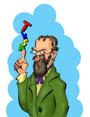
Ludwig Boltzmann
A Mild Resemblance
Everyone in the world clamors for a demonstration on how to derive the famous Boltzmann Distribution. After all, if the whole world understood this simple principle, ignorance and superstition, would be eradicated forever!
So to help eradicate ignorance and superstition we must retrace the thinking - and the life and times - of Ludwig Boltzmann.
And just who was Ludwig Boltzmann?
Ludwig was a nineteenth and early twentieth century German professor of physics who bore a mild resemblance to Edwin Stanton, the Secretary of War under Abraham Lincoln. Or maybe he favored famed musician Leon Russell.
Actually Ludwig was from Austria, not Germany. He was born in Vienna in 1844, and his situation was fairly comfortable. His dad was a government official and so Ludwig was able to enter the gymnaisum (pronounced "gim-NAHS-ee-um" with a hard "g"). This was a particularly tough college preparatory school which compensated for the fact that in some ways the 19th century university curriculum was more lackadaisical than today. In any case, Ludwig graduated at the top of the gymnasium and entered the University of Vienna.
He studied both mathematics and physics and graduated with a Ph. D. in 1866. However, at that time in Germany a Ph. D. and fünf pfennigs could buy you eine Tasse Kaffee. To teach in a university you had to have a Habilitation. This was (and is) a sort of super-degree but one was that awarded based on scholarly contributions. With a Habilitation in his pocket, Ludwig was hired by the University of Graz.
Except for one interlude, Ludwig seemed to be inflicted with Wanderlust. After four years in Graz, he was hired by the University of Vienna as Professor of Mathematics. But that stay was also brief and he returned to Graz, in part we think because it was there he met a young lady, Henriette Magdalena Katharina Antoniavon Edle von Aigentler. For obvious reasons, Ludwig called her "Jetti".
As a girl, Henriette had been interested in physics and mathematics. But at the time, women were either not allowed in the universities or at least strongly discouraged from pursuing "masculine" studies that (the men thought) would send the ladies into hysteria and infirmity, if not madness and sterility.
Ludwig, though, seemed to have appreciated the problems women faced when breaking out of the Kinder, Küche, Kirche Unsinn that was de rigueur in Deutschland (and all other countries for that matter). All his life Ludwig was happy to have the ladies attend his classes and that included Henriette.
Ludwig's return to Graz was a rather complex matter as he was competing for the Chair of Experimental Physics with Ernst Mach. You'll read that Ludwig and Ernst didn't get along but this seems to have been more professional disagreements rather than personal enmity. Certainly Ernest helped promote his younger colleague's career and stepped aside to let Ludwig take the post at Graz. Ernst then went to the University of Prague where he taught for the next eighteen years.
Ludwig stayed in Graz from 1876 to 1890 - his most lengthy stay at any school. He married Henriette and they had five kids.
By the mid 1870's, Ludwig had developed a solid reputation as a physicist. His specialty was the new field of statistical mechanics (which he is often credited with inventing). But it was in latter years at Graz that he began to suffer from what was called "neurasthenia".
Like many 19th century diseases, this is a rather ill-defined condition but is characterized by irritability, fatigue, and depression. It was one of these "attacks" that seems to have cost him a professorship at the University of Berlin in 1888.
Today we would say Ludwig suffered from what we would call an extreme bipolar disorder or in older terms, severe maniac-depressive illness. Of course, the years after 1880 were not easy times for Ludwig. His mom had died in 1884 and his sister in 1890.
But it was probably the death of his son from appendicitis in 1885 that prompted Ludwig to leave Graz. At that time he was one of the most famous physicists in the world, and knew he would have no problem landing a job elsewhere. So in 1890, he went to the University of Munich.
At Munich Ludwig's lectures were popular with the students who were used to dry unenthusiastic droning. He had a number of friends on the faculty, and he seems to have had a good social life. Word was he tubbed up on the good Bavarian cuisine.
The trouble was that the University of Munich offered no pensions and one of the more famous former professors ended up dying in poverty. So in 1894, possibly with the prompting of Henriette, they returned to the University of Vienna which seems to have been a bit more generous to its faculty.
At Vienna Ludwig again found himself popular with the students and he encouraged women to attend his classes. One of his students was Lise Meitner who later discovered the theory of nuclear fission.

Lise Meitner
A Student
Ludwig's big academic battle was about atoms, and whether they existed or not. A lot of people thought they were just mathematical conveniences - like the epicycles used in the equations for the solar systems that used circular rather than elliptical orbitals. Even able and well-known scientists - including Ernst Mach - weren't convinced. But Ludwig believed atoms were real and most of his research was based on what happened with atoms bouncing around.
The biggest boost for atomism - as it was called - came in 1905 when Albert Einstein published a paper that demonstrated Brownian Motion - the jiggling of pollen grains or soot particles in water - was best explained by the actual existence of tiny particles bouncing around and smacking against the pollen or soot. Although Albert's paper didn't convince the die-hard hold-outs, by the early 20th century, most everyone agreed atoms existed.
Ludwig's eyesight had begun to deteriorate although in early 1906 he had been able to visit America where he lectured at Berkeley. He returned to Vienna for the summer and in November he was vacationing with his family when he hanged himself.
The Boltzmann Derivation
Easier Than It Looks
Ludwig, we must say, did not invent thermodynamics. The laws of thermodynamics had been worked out over a period of about a century and a half. The basic laws deal with heat transfer and are independent of any atomic theory. But if atoms are real, then they must be responsible for thermodynamics.
And it's how the atoms and molecules create heat and make heat flow around that statistical mechanics tries to explain. Specifically, it is the velocity of the atoms and molecules and so the energies of the molecules that dictate how the heat flows.
And Ludwig set out to calculate how the molecules' velocities and energies change. Although seemingly a formidable task, actually it's easier than it looks. That is, provided we don't try to do too much.
So we'll go through the basics of what Ludwig did - although James Clerk Maxwell - the middle name is pronounced "clark" - is also given credit for the discoveries.
Now in a box of molecules you can only have so many of them. And each molecule will have an energy. So to get the total energy, all you have to do is sum up the energies of the individual molecules.
If we have 602,250,000,000,000,000,000,000 molecules, the total energy is just:
| Energy |
|
= |
|
εMolecule 1 + εMolecule 2 + εMolecule 3 + εMolecule 4 + ... + εMolecule 602250000000000000000000
|
Unfortunately, we don't know what any of the εMolecule i values are. But that's where Ludwig stepped in.
Ludwig saw it was too much trouble to keep track of all of the molecules. So he said he'd just consider groups of them. And he would group the ones together that had the same energy.
But hold on there, you say. You can't assume even a few molecules have the same energy. The energy of a molecule depends on its speed. And since speed can be any real number there are an infinite number of possibilities!
Well, that's true, but not a problem. Instead we will create artificial and equally spaced bins of energies. And we will then assign each molecule to the bin which has the value closest to its energy. Then we just count the number of molecules in each bin.
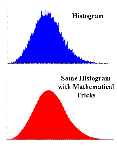
Histograms
Mathematical Tricks
In other words, we make a histogram of the molecules and their energies.
The trouble is histograms are rather jagged and irregular. But since the numbers are rather arbitrarily grouped, they only show an approximate relationship between the numbers.
On the other hand, there are various mathematical tricks to take the jagged histogram and turn it into a nice smooth curve that will let the molecules reassume their individual identities and their own energy. And that's what Ludwig did.
OK. We have our molecules in each bin which are assigned an energy value.
| nk | | εk |
| : | | : |
| n3 | | ε3 |
| n2 | | ε2 |
| n1 | | ε1 |
So it's clear the energy of the whole system must be:
| Energy |
|
= |
|
n1ε1 + n2ε2 + n3ε3 + n4ε4 + ... + nkεk
|
... which is written more compactly as:
... where Σ is the summation sign.
Obviously, the total number of molecules, 602,250,000,000,000,000,000,000, is given by:
|
|
ni |
= |
|
602,250,000,000,000,000,000,000, |
|
|
... and is constant.
For simplicity we'll let:
602,250,000,000,000,000,000,000 = N
... and our equation for the total molecules is just:
Now it turns out that not all distributions occur as often as others. We can get an idea why this is so by considering a very simple system: one with only three molecules and two energy levels:
| Number | Level 1 | Level 2 |
1 | mmm | |
2 | mm | m |
3 | m | mm |
4 | | mmm |
We see there are four different arrangements - that is four different configurations. And since there is only one of each of the configurations, you might think they are equally likely to form. That, though, is not correct.
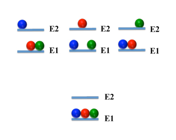
Distributions
(Click Image to Open in Larger Window)
Instead, we can see - if you click on the image to the left - that there is only one way to pack the molecules into the first level. But there are three ways to put one molecule in the second level and the two others in the first. So this state is three times more likely to occur than the one where all molecules are in the same level.
Of course if we are talking about molecules we have a lot more than three of them and we also have a lot more than two energy levels. So what we need is a general equation for calculating the number of configurations or microstates.
Well, with billions and billions of molecules, we obviously don't have the time to draw a diagram like the one we had above. Instead, we turn to a field of mathematics called combinatorics which comes to the rescue.
Now at some time everyone has heard about the problem of how to put balls into boxes. But putting molecules into energy levels is exactly the same.
There are various scenarios: distinguishable balls and distinguishable boxes, indistinguishable balls and distinguishable boxes, distinguishable balls and indistinguishable boxes, and indistingiushable balls and indistinguishable boxes. You can have more boxes than bins and more bins than boxes - or even the same number of bins and boxes. You can allow some boxes to be empty or require all of them to be filled. The options are legion.
In our case, though, we will impose no restrictions on the energy levels except we have at least as many levels as molecules. And they can be filled or not as we choose. Our only restriction is we have a fixed number of balls (ergo, molecules).
With these stipulations, the combinatorialists tell us that starting with N balls (molecules), the total number of ways to put our them into the bins (energy levels) is:
| W |
|
= |
|
N × (N - 1) × (N - 2) × ... × 2 × 1 |
|
... where W is the Ways of filling the energy levels.
And for those who have had middle school math, you will recognize the product at the right of the equals sign as the factorial of N. This is written in compact form as:
W = N!
So we see that if you have three molecules packed into one energy level, there are
3 × 2 × 1 = 6
... ways to put the molecules in the level.
But hold on again! We said there was only one way to pack all three molecules into one level. How do you explain that?
Now it's important to realize the equation, W = N!, treats the molecules as if they are distinguishable. That is if you make each ball a different color, one blue (B), one green (G), and one red (R), we see we do indeed have:
| B |
G |
R |
| B |
R |
G |
| R |
B |
G |
| R |
G |
B |
| G |
B |
R |
| G |
R |
B |
3! = 6 ways or permutations to fill the level with multicolored balls.
So why do we say there was only one way to fill the level with molecules?
The reason is that molecules are not distinct balls. Molecules are indistinguishable. And so our equation W = N! has overcounted the ways we can pack them in the energy levels.
And how do we make the correction?
That's very easy to do. You just take the factorial of the number of molecules in a particular energy level - which is ni!. That's the number of ways you can rearrange the molecules in the level. We then just divide this number into N! and get corrected number of permutations or combinations.
It certainly works for the case where there's only one energy level and 3 molecules. After all there is indeed 6!/6! = 1 way to pack the indistiguishable molecules in.
The general case, then, is if we have ni molecules in a given Level i, then there are
ni × (ni - 1) × (ni - 2) × ... × 2 × 1 = ni!
... distinguishable permutations. And so to correct for the overcounting of this level we divide N! by ni!.
Corrected W (for Level i) = N!/ni!
But our molecules are distributed over many energy levels. So we make the same type of correction for all energy levels. That is, we divide N! - the total permutations of the total molecules - by the product of the permutations of the molecules in all energy levels.
n1! × n2! × n3! × ... × n(k - 1)! × n(k - 1)!
... which means the total number of configurations - corrected for the indistinguishably of the molecules - is:
| W |
|
= |
|
| N! |
|
| n1! × n2! × n3! × ... × n(k - 1)! × n(k - 1)! |
|
Notice that we list all energy levels in the denominator. But some of them may be empty. So how do we handle this?
Well, we don't need to. That's because the factorial of 0, 0!, is 1.
0! = 1
... so you never divide by zero, even if there's no molecules in an energy level and we don't know the number of energy levels. This formula even works if we have an infinite number of empty energy levels. Pretty slick.
We have to make it clear that what we have is a formula for calculating the ways to make one particular configuration. That is, if we know the total number of molecules and the number of ways the molecules are distributed in the energy levels, we can count the total number of ways that particular configuration can arise.
For instance, say we have 10 molecules and 5 of these are in energy Level 1, 3 of them in energy Level 2, 2 in Level 3, and none in Level 4 or higher. How many distinct configurations of these do we have?
Well, just plug in the numbers.
| W |
|
= |
|
| 10! |
|
| 5! × 3! × 2! × 0! ... × 0! |
|
| |
|
= |
|
| 3628800 |
|
| 120 × 6 × 2 × 1 ... × 1 |
|
| |
|
= |
|
|
| |
|
= |
|
2520 |
So far so good. But now we want to find - not just how the molecules can distribute themselves - but how the molecules will distribute themselves in the most probable manner. After all, that's what the molecules will do when they are at thermal equilibrium.
This is simple - with a bit of calculus. We just optimize W to find it's maximum value. And to do that we take the derivative of W with respect of all values of ni. Set the derivative equal to zero, and solve for each values of ni.
| ∂W |
|
| ∂n1∂n2∂n3...∂nk-2∂nk-1∂nk |
|
|
|
= |
|
|
|
0 |
|
Yes, that's all we have to do.
Sadly, a little experimentation will show that taking a derivative of factorial expressions is a lot of work. But fortunately, the mathematicians of the 18th and 19th century had been developing all sorts of tricks. Specifically they found you can save a lot of time by working with the natural logarithm of W rather than W itself.
That is, we will work with:
| lnW |
|
= |
|
|
|
ln ( |
|
|
|
|
|
| N! |
|
| n1! × n2! × n3! × ... × nk - 1! × nk! |
| |
|
) |
|
... which the rules of logarithms simplifies the equation to:
lnW = lnN! - ln(n1! n2!n3! ... nk - 1!nk!)
... and even simpler once we write everything as addition and subtraction:
lnW = lnN! - (lnn1! + lnn2! + lnn3! ... lnnk - 1! + lnnk!)
You'll notice that to avoid a multiplicity of parentheses we will write the natural logarithm - usually written like ln(x) - simply as lnx. So expressions like ln(W), ln(N), and ln(ni) are the same as lnW, lnN, and (as we just wrote) lnni.
We can see, then, that by using the summation sign, Σ, our new equation can be written with even greater succinctness:
... where k is the number of energy levels.
Now at this point you may ask, what's the point? You say it's hard to take the derivative of a factorial. But look what we have now! We still have the factorials and we've added logarithms. So we now have two functions to differentiate!
But fortunately, the 18th century mathematicians show us how to get rid of the factorials. We do this by approximating the logarithm of the factorial. In particular, we use Stirling's Approximation for Lnx!.
lnx! = xlnx - x
This gives an error of less than 1 % if x > 90.
So with a little middle school algebra we began to transform our equation which is:
...and by substituting all logarithms with Stirling's Approximation we continue:
| lnW |
|
= |
|
(NlnN - N) |
|
- |
|
|
(nilnni - n) |
| |
|
= |
|
NlnN - N |
|
- |
|
|
nilnni + |
|
ni |
| |
|
= |
|
NlnN - N |
|
- |
|
|
nilnni + |
N |
| |
|
= |
|
NlnN |
|
- |
|
|
nilnni + |
- N + N |
| |
|
= |
|
NlnN |
|
- |
|
|
nilnni |
... and we end up with a bit simpler equation:
Since we're working with logarithms, our goal is to optimize lnW rather than W.
| ∂lnW |
|
| ∂n1∂n2∂n3...∂nk-2∂nk-1∂nk |
|
|
|
= |
|
|
|
0 |
|
And to make it even easier, we will do something that will vex calculus teachers. We will use, not the full derivatives, but instead just the differential.
dlnW = 0
A problem with using differentials is that when applied to the variables rather than the functions is that they they don't just become a differential. They become infinitesimals.
Now during the 20th-century it became common for calculus teachers to spit on the ground about infinitesimals. "We don't work with infinitesimals anymore," a professor once sniffed with hauteur. Instead they stress that they work with limits and numerical neighborhoods like |x + ε| and |f(x) + δ| which is way to teach calculus that everyone agrees no one can understand.
This anti-infinitesimal stance is pretty funny since in the 1960's it was proven that infinitesimals are perfectly valid and rigorous mathematical entities. They are in fact an extension of the real number system much like real numbers are an extension of the rational numbers. You can read about hyperreals and how they let use legitimately use infintessimals if you just click here.
So armed with infinitesimals and their big cousins the differential, we start off by taking the differential of Stirling's Approximation of lnW.
| dlnW |
|
= |
|
d (NlnN |
|
- |
|
|
|
|
|
|
nilnni) |
| |
|
= |
|
d(NlnN) |
|
- |
|
|
|
|
d ( |
|
nilnni) |
Now the first thing to remember is that if C is a constant, then the differential expression, dC, is zero. Since N is a constant, so is NlnN. So we can write for the first term:
d(NlnN) = 0
And so our equation becomes:
At this point we have to use the product rule of derivatives (and differentials). You learned this in calculus classes and if f and g are functions, then the differential of their product d(fg) is given by:
d(fg) = f(dg) + g(df)
... and so our differential for the expression within the summation sign, d(nilnni), is:
d(nilnni) = nid(lnni) + lnnidni
... and this equation can be transformed to:
| d(nilnni) |
|
= |
|
nid(lnni) + lnnidni |
|
|
|
= |
|
(1 + lnni)dni |
|
Now it may not be obvious where the "1" came from. That's from a bit of calculus gymnastics which is worth explaining.
First to make the equations a bit easier to manipulate, we'll substitute x for ni and take the derivative - yes, the derivative - of xlnx:
d(xlnx)/dx = x(dlnx/dx) + lnx(dx/dx)
So we now look up the derivative for dlnx:
dlnx/dx = 1/x
... and since we know that:
dx/dx = 1
... and by plugging these values in the expression for d(xlnx)/dx, we get:
| d(xlnx)/dx |
|
= |
|
x(1/x) + lnx(1) |
| |
|
= |
|
1 + lnx |
... and we've shown:
Since by definition of the dg, that is, the differential of the function, g(x)
dg = (dg/dx)dx
... then for the function xlnx:
| d(xlnx) |
|
= |
|
(d(xlnx)/dx)dx |
| |
|
= |
|
(1 + lnx)dx |
Now we let's resubstitute ni for x:
| d(nilnni) |
|
= |
|
nid(lnni) + lnnidni |
|
|
|
= |
|
(1 + lnni)dni |
|
and our equation for dlnW is:
That's where the "1" comes from.
So now we can continue:
| dlnW |
|
= |
- |
|
(1 + lnni)dni |
|
| |
|
= |
- |
|
(dni + lnnidni) |
|
| |
|
= |
- |
|
dni - |
|
lnnidni |
Now at this point you have to remember that:
... but that since N is constant...
dN = 0
... and therefore:
... and our final equation for dlnW becomes:
Or rather that's nearly our last equation for dlnW.
We mentioned that the 18th and 19th century was a time when mathematicians were discovering new ways to do calculations. And a lot of the new calculations were perfect for the physicists. But that's not surprising since sometimes the mathematicians and the physicists were the one and the same.
One of the most important of these mathematical physicists was Joseph Louis Lagrange, most famously known for creating the lazy man's coordinate system. But in this case we'll borrow a method he developed for optimizing functions where the function was subject to constraints.
Constraints are needed in physical sciences. That's because in the real world physical quantities can't be any value. You don't have negative weights, for instance. So you have to make sure your equations are restricted to reality.
In our case we have the constraints that the total energy and the number of our molecules are constant. So how do we work these contraints into our equation?
Well, Joseph Louis was a true genius. He knew that 0 plus 0 is equal to 0.
0 = 0 + 0
So if a function is equal to zero you can add any number of functions that are also equal to zero and not change the value. So Joseph Louis developed a method he called the Lagrange Method of Undetermined Multipliers.
With Joseph Louis's method you have a function, F, you need optimized. So of course you take the derivative and set it equal to zero.
dF/dx = 0
But suppose you have some constraints on F that can also be written as functions equal to zero:
g(x) = 0
h(x) = 0
You can add these functions to the derivative and not change the value:
dF/dx + g(x) + h(x) = 0
But note you can also multiply the added functions by constants - we'll call them α and β - and the products still equal zero. After all, a constant times zero is still zero:
αg(x) = 0
βh(x) = 0
And you can add the functions times the constants to your equation ...
dF/dx + αg(x) + βb(x) = 0
... or subtract them:
dF/dx - αg(x) - βb(x) = 0
... and our equation still works.
It seems we're making things more complicated, not less. But what we're doing is making our function and it's constraints tied up in one nice neat equation. This actually simplifies things.
For instance we can now write our equation - we'll use the negative constants - in differential form:
(dF/dx)dx - αg(x)dx - βb(x)dx = 0
... which is the same as:
(dF/)dxdx = αg(x)dx + βb(x)dx
... and
dFdx = αg(x)dx + βb(x)dx
... which you'll recognize as a nice integrable equation:
... which has our constraints built in.
And in our problem?
Remember we have two constraints.
First the total energy does not change. So the change in total energy, dE, is zero.
dE = 0
And since:
And taking the differential dE.
| dE |
|
= d( |
|
εini) |
|
| |
|
= |
|
εidni |
|
| |
|
= |
0 |
Secondly, the total number of molecules, N, is constant. That means:
dN = 0
And using the equivalent expression:
So our two constraints can now be listed as:
Since the functions dN and dE are both equal to zero we can add them to our function for dlnW. And we can multiply them by the two constants and not change the value for dlnW.
So as we continue:
| dlnW |
|
= |
- |
|
lnnidni |
|
| |
|
= |
- |
|
lnnidni |
| + α |
|
|
dni |
lnnidni |
| - β |
|
|
dεdni |
... where the signs of our constants, α and β, are selected for convenience.
Now we know when lnW is at an optimum (maximum), then dlnW = 0.
So we have:
| 0 |
|
= |
- |
|
lnnidni |
| + α |
|
|
dni |
lnnidni |
| - β |
|
|
εdni |
Or a bit simpler:
| 0 |
|
= |
- |
|
(-α + βεi + lnni)dni |
|
Now there are two ways a summation series can equal zero. One way is to have pairs of terms that are equal in value but opposite in sign. The other way is to have all terms equal zero. Our series fits the last type and each term in our summation must equal zero.
Since each individual term equal zero, for now we can dump the summation sign and consider only an individual term for a particular energy level:
0 = -α + βεi + lnni
... and with some very minor algebra:
lnni = α - βεi
... and writing the logarithm equation in exponential form:
| ni |
|
= |
|
e(α - βεi) |
|
|
= |
|
eαe-βεi |
|
So our horribly complex equation filled with factorials, ratios of factorials, and logarithms of factorials ends up being a quite simple function. That is ...
ni(εi) = eαe-βεi
... gives the number of number of molecules with energy εi.
Remember that this equation was formed by looking at a single term of the summations. So we need to put back the summation.
And we also know that:
... and therefore:
You can see that we are now close to getting away from the artificial concept of molecules in bins. To complete this transition we realize we are working with a huge number of molecules and even more closely spaced energy levels. So we can replace the summation sign, Σ, with an integral, ∫.
Note that our summation over k begins with k = 1. But k is just an index of the bins. In the integrals we replace k with the actual value of εk. And the lowest energy value is zero.
And the highest value? Well, there is no upper limit.
So we end up with a definite integral of an exponential function of ε which we integrate from 0 (the lowest possible value) to infinity.
So we start off:
| N |
|
= |
|
|
n(ε)dε |
| |
|
= |
|
|
eαe-βεdε |
| |
|
= eα |
|
|
e-βεdε |
And since we know by looking it up:
So making the appropriate substitutions:
So we have shown:
N = eα/β
... which means:
eα = βN
And so we can now write our optimized equation quite simply as:
So if we divide both sides of the equation by N we get:
Which with very minor rearrangement gives us:
So what, as Flakey Foont asked Mr. Natural, does it all mean?
Notice we now have a function, βe-βε, which 1) is positive for all values of ε, and 2) whose integral from 0 to ∞ equals 1.
In other words, the formula, βe-βε is a probability function which we can abbreviate as: P(ε):
P(ε) = βe-βε
We derived P(ε) from the number of molecules. But we would get the same probability function for any other property that was dependent on energy and which we had optimized for distribution among the energy values. So P(ε) works for other molecular properties as well.
One of the reasons to calculate a molecular or atomic probability function is to calculate the expectation value of a property that arises from the molecules or atoms.
To do that we just multiply the value of the molecular or atomic property by the probability function. We then integrate from 0 to ∞.
And the general equation for the expectation value when you have a probability function is:
... where <X> is the expectation value of Property X and x(ε) is the value of the property at the particular value of ε
In short, the expectation value is just the average. That is, the value of the property that we would actually measure.
Since we don't know what β is - even Ludwig didn't know it - we can't give an exact value of how the molecules fill the energy levels.
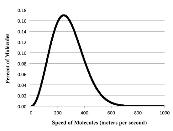
But we can look at the general shape of the curve. For instance, for P(ε), the probability curve itself, we'll set β = 0.25 and plot it out from 0 to 25.
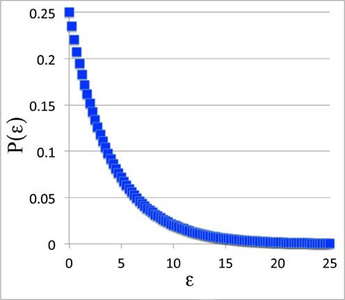
The Probability Function:
Just Part of the Answer
(Click on Graph to Open
in a Separate Window)
All right. This doesn't look much like the Boltzmann distribution. Did we do that work for nothing? Was Mr. Natural correct after all?
Well, let's look at the expectation value instead. Or rather let's look at the function we integrate to get the expectation values. We'll call that new function D(P)
D(P) = xP(ε) = x(ε)βe-βε
D(P) is called the probability density function. This is the probability function times the value of the property.
Note that at zero, the probability function is zero, no matter how large P(ε) is. But as x(ε) gets larger P(ε) gets smaller. So we get a balancing act and the curve of the density function itself can rise and fall.
But does it? Well for a specific example, let's just use the energy value itself, ε. That is:
x(ε) = ε
...and so we plot:
D(P) = εβe-β ε
... which is:
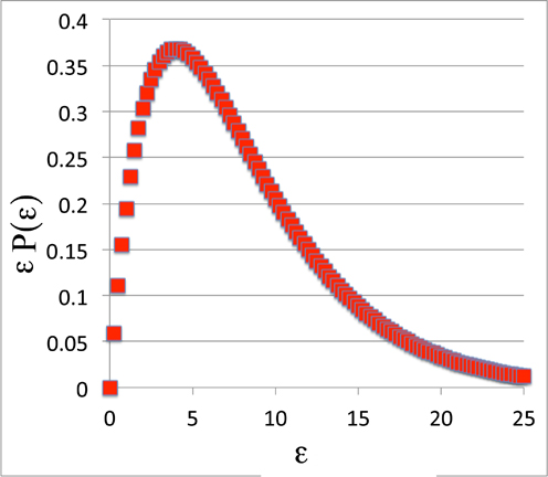
The Probability Density Function:
Looks Familiar
(Click on Graph to Open
in a Separate Window)
Yep. It's the Boltzmann Distribution itself!
How about that?
Ludwig did not just come up with the most probable way molecules spread out their energy. During his work he hit upon a more fundamental concept that everyone has heard of but not many really understand.
Remember Ludwig started off with the equation:
| W |
|
= |
|
| N! |
|
| n1! × n2! × n3! × ... × n(k - 1)! × n(k - 1)! |
|
... and this represents the ways you can arrange the molecules. Each arrangement is called a microstate.
And also remember that part way through our derivation we had the equation:
Since we're working with logarithms, our goal is to optimize lnW rather than W.
| ∂lnW |
|
| ∂n1∂n2∂n3...∂nk-2∂nk-1∂nk |
|
|
|
= |
|
|
|
0 |
|
... which leads to a probability function that would apply to any property that was related to the energy of the system.
So Ludwig realized that lnW itself represented a fundamental property of a system. Or rather lnW was proportional to the property, and he came up with a quite simple and his most famous equation:
S = klnW
... where k is a constant.
Now as we said, W is not necessarily the ways of arranging molecules but the ways of arranging the microstates of the system. The system can be molecules in a box, but it doesn't need to be. Other things that define a system can be used to calculate S. Ludwig dubbed S the entropy.
Today entropy is recognized as one of the fundamental thermodynamic properties of nature. But it is also used to describe a number of concepts that have something akin to the S = klnW formula. Entropy functions are used not just in physics and chemistry but in other fields as diverse as medicine, cryptography, information theory, computer science, and sociology.
The importance of entropy was it is a measure of how initial low probability microstates will tend toward higher more probable arrangements and it is unlikely they will return to an original low probability state. For instance, if you blow up a balloon and let the air out, it isn't likely that the air in the room will by itself and by chance fill up the baloon again. It's not impossible, mind you, just not very likely.
But one thing to remember - as we want to combat ignorance and superstition - is that it is not true that ordered and complex systems cannot form spontaneously in nature and that spontaneous formations of order are against the laws of thermodynamics. Spontaneous organization happens all time.
The false belief that you hear spouted on the Fount of All Knowledge - and in (regrettably) some schools - is that spontaneous processes of a system occur only with an increase in entropy of the system. Since an increase in entropy is one of less order, they say anything of high order forming spontaneously cannot occur without something operating outside the laws of nature.
That is, we should say, complete horse hockey, bullshine, and poppycock.
What is true is for a spontaneous processes the sum of the entropy change of the system plus the entropy change of the surroundings will be greater than zero. And this does not mean a system can not spontaneously become more ordered.
Instead as long as a system evolves sufficient heat which is dispersed to the surroundings, the system can become more ordered and less random. In fact, using using only (literally) grade school math, you can prove that as long as the heat transmitted to the surrounding is greater than the temperature multipled by the loss of entropy (which has units of energy per degree), the surroundings will gain sufficient entropy so the system can become more ordered.
But hold on, say The Credulous. Are you saying that when ice freezes spontaneously on a winter's day, the ice actually gives off heat?
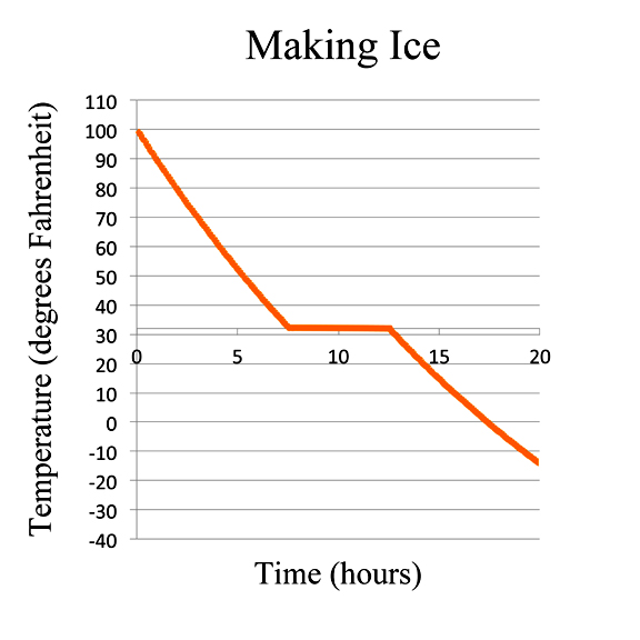
Ice Melts aka Eradicating Ignorance and Superstition
(Click on Graph to Open
in a Separate Window)
Yep. That's exactly what happens. In fact, when a gallon of water freezes, it gives off about 33 food-calories of energy. That's as much energy you get if you eat about 2½ tablespoons of fat.
This is why if when the temperature drops and water starts cooling down, the temperature follows a nice smooth curve until the water starts to freeze. Then as the water begins to loose its disorder - ego, the ice forms - the formation of the ice crystals produces heat. The evolution of heat is the reason the ice/water mixture stays at a constant temperature as it freezes. And the heat transmitted to the surroundings produces an increase in entropy in the surroundings which is at least as large as the decrease in entropy of the water.
This transfer of heat to the surroundings is the basis for all natural processes by which complex structures are formed. It doesn't matter if it's crystal formation or the formation and replication of living cells. The time required is irrelevant and even applies to the universe as a whole. As the universe continues to expand the total entropy will increase, but the disorder of individual systems - planets, stars, solar systems, and even galaxies - will decrease.
The main lesson from Ludwig's discovery of statistical entropy is that an increase in entropy is an increase in the availability of the energy levels. It may (or may not) be associated with physical order or disorder.
To close up we'll mention that the famous modern representation of Ludwig's equation - often called the Maxwell-Boltzmann Distribution - is more complex and it varies depending on who does the deriving. Also the Boltzmann's constant is also written as k = Temperature × β. The β we derived isn't the same as the modern β.
The Boltzmann's constant, k, has a value of:
1.38064852 × 10⁻²³ joules per degrees Kelvin
... which in more household units is:
1.83203 × 10⁻²⁷ food-calories per degrees Fahrenheit
The modern Boltzmann's constant is, in fact, the famous Avagadro's Gas Constant, usually designated R, divided by Avagadro's Number, 602,250,000,000,000,000,000,000. The modern Boltzmann constant wasn't defined until 1900.
And by whom?
Max Planck!
References
Ludwig Boltzmann His Later Life and Philosophy, 1900-1906: Book One, John Blackmore (Editor), Springer, 1995.
Lise Meitner: A Life in Physics, Ruth Lewin Sime, University of California Press (1996).
"The Misinterpretation of Entropy as 'Disorder'", Frank Lambert,
J. Chem. Educ., 2012, 89 (3), pp 310-310, 2012.
Return to Ludwig Boltzmann Caricature
Return to CooperToons Caricatures
Return to CooperToons Homepage